2.4 Paleomagnetism and Sea Floor Spreading
Steven Earle and Laura J. Brown
As the mineral magnetite (Fe3O4) crystallizes from magma, it becomes magnetized with an orientation parallel to that of Earth’s magnetic field at that time. This is called remnant magnetism. Rocks like basalt, which cools from a high temperature and commonly have relatively high levels of magnetite (up to 1 or 2%), are particularly susceptible to being magnetized in this way. Still, as long as they have small amounts of magnetite, even sediments and sedimentary rocks will take on remnant magnetism because the magnetite grains gradually become reoriented following deposition. By studying both the horizontal and vertical components of the remnant magnetism, one can tell the direction to magnetic north at the time of the rock’s formation and the latitude where the rock formed relative to magnetic north.
In the early 1950s, a group of geologists from Cambridge University, including Keith Runcorn, Ted Irving, (Ted Irving later set up a paleomagnetic lab at the Geological Survey of Canada in Sidney, B.C., and did a great deal of important work on understanding the geology of western North America) and several others, started looking at the remnant magnetism of Phanerozoic British and European volcanic rocks and collecting paleomagnetic data. They found that rocks of different ages sampled from generally the same area showed quite different apparent magnetic pole positions (Figure 2.8). They initially assumed that this meant that Earth’s magnetic field had, over time, departed significantly from its present position—which is close to the rotational pole.
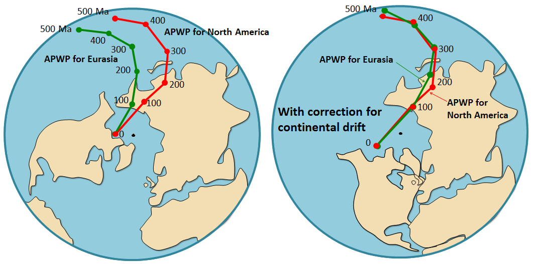
The curve defined by the paleomagnetic data was called a polar wandering path because Runcorn and his students initially thought that their data represented the actual movement of the magnetic poles (since geophysical models of the time suggested that the magnetic poles did not need to be aligned with the rotational poles). We now know that the magnetic data define continents’ movement, not of the magnetic poles, so we call it an apparent polar wandering path (APWP).
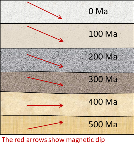
At around 500 Ma, what we now call Europe was south of the equator, and so European rocks formed then would have acquired an upward-pointing magnetic field orientation (see Figure 2.9). Europe gradually moved north between then and now, and the rocks forming at various times acquired steeper and steeper downward-pointing magnetic orientations. When researchers evaluated magnetic data in this way in the 1950s, they plotted where the North Pole would have appeared to be based on the magnetic data and assumed that the continent was always where it is now. That means that the 500 Ma “apparent” north pole would have been somewhere in the South Pacific and that it would have gradually moved north over the following 500 million years. Of course, we now know that the magnetic poles don’t move around much (although polarity reversals do take place). Europe had a magnetic orientation characteristic of the southern hemisphere because it was in the southern hemisphere at 500 Ma. Runcorn and colleagues soon extended their work to North America, which also showed apparent polar wandering, but the results were inconsistent with those from Europe. For example, the 200 Ma pole for North America was plotted somewhere in China, while the 200 Ma pole for Europe was plotted in the Pacific Ocean. Since there could only have been one pole position at 200 Ma, this evidence strongly supported the idea that North America and Europe had moved relative to each other since 200 Ma. Subsequent paleomagnetic work showed that South America, Africa, India, and Australia also have unique polar wandering curves. In 1956, Runcorn changed his mind and became a proponent of continental drift. This paleomagnetic work of the 1950s was the first new evidence in favour of continental drift, and it led several geologists to start thinking that the idea might have some merit. Nevertheless, for most geologists working on global geology at the time, this type of evidence was not sufficiently convincing to get them to change their views.
During the 20th century, our knowledge and understanding of the ocean basins and their geology increased dramatically. Before 1900, we knew virtually nothing about the bathymetry and geology of the oceans. By the end of the 1960s, we had detailed maps of the topography of the ocean floors, a clear picture of the geology of ocean-floor sediments and the solid rocks underneath them, and almost as much information about the geophysical nature of ocean rocks as of continental rocks.
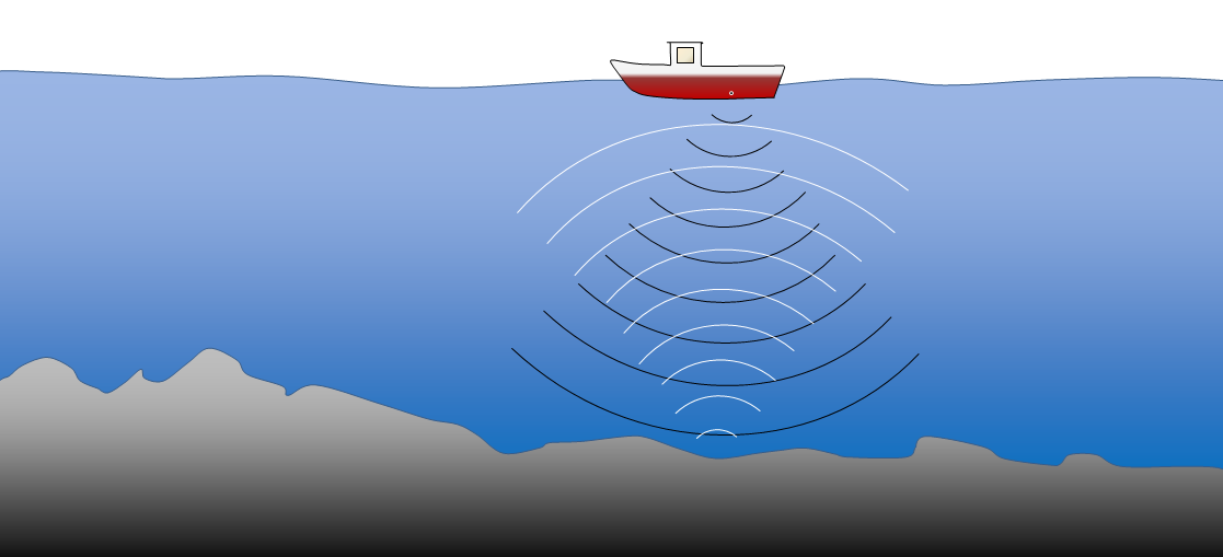
Up until about the 1920s, ocean depths were measured using weighted lines dropped overboard. This is a painfully slow process in deep water, and the number of soundings in the deep oceans was probably fewer than 1,000. That is roughly one depth sounding for every 350,000 square kilometres of the ocean. To put that in perspective, it would be like trying to describe the topography of British Columbia with elevation data for only half a dozen points! The voyage of the Challenger in 1872 and the laying of trans-Atlantic cables had shown that there were mountains beneath the seas. However, most geologists and oceanographers still believed that the oceans were essentially vast basins with flat bottoms filled with thousands of metres of sediments.
Following the development of acoustic depth sounders in the 1920s (Figure 2.10), the number of depth readings increased by many orders of magnitude. By the 1930s, it had become apparent that major mountain chains existed in the world’s oceans. There was a well-organized campaign to study the oceans during and after World War II. By 1959, sufficient bathymetric data had been collected to produce detailed maps of all the oceans (Figure 2.11).
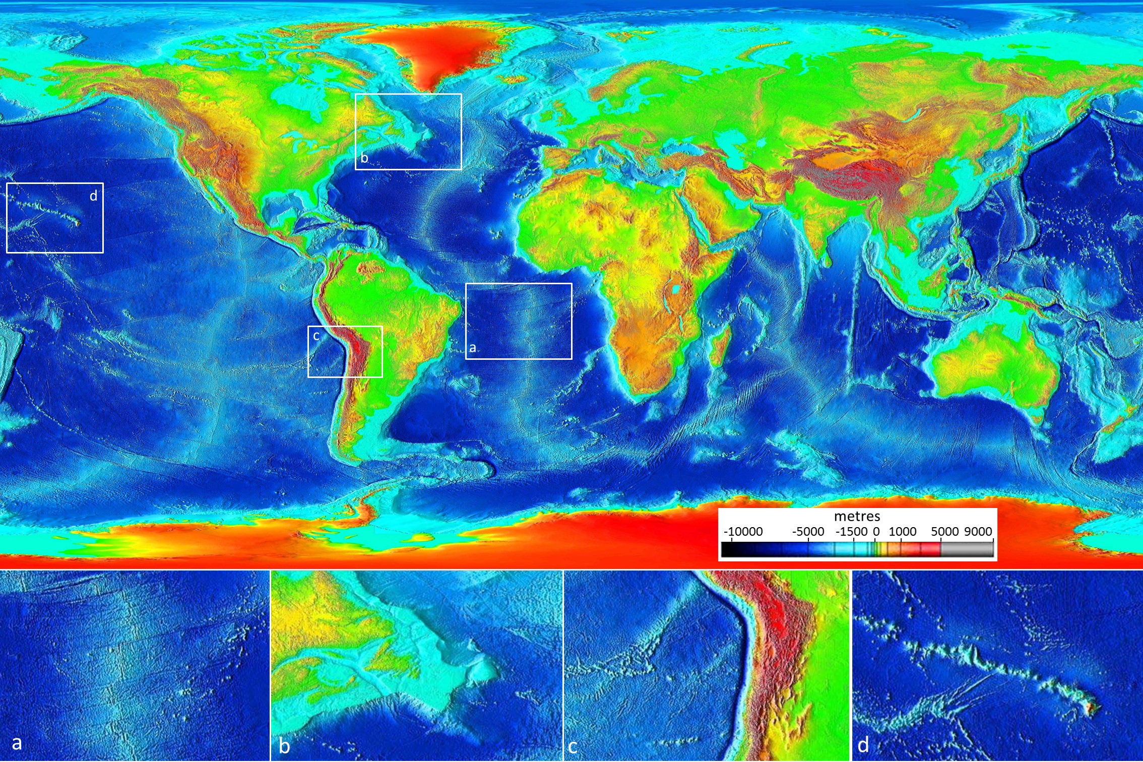
The important physical features of the ocean floor are:
- Extensive linear ridges (commonly in the central parts of the oceans) with water depths in the order of 2,000 to 3,000 m (Figure 10, inset a)
- Fracture zones perpendicular to the ridges (inset a)
- Deep-ocean plains at depths of 5,000 to 6,000 m (insets a and d)
- Relatively flat and shallow continental shelves with depths under 500 m (inset b)
- Deep trenches (up to 11,000 m deep), most near the continents (inset c)
- Seamounts and chains of seamounts (inset d)
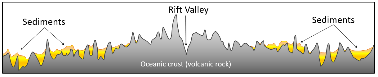
Seismic reflection sounding involves transmitting high-energy sound bursts and then measuring the echoes with a series of geophones towed behind a ship. The technique is related to acoustic sounding as described above; however, much more energy is transmitted, and the sophistication of the data processing is much greater. As this technique evolved and the amount of energy was increased, it became possible to see through the sea-floor sediments and map the bedrock topography and crustal thickness. Hence sediment thicknesses could be mapped. It was soon discovered that although the sediments were up to several thousand metres thick near the continents, they were relatively thin — or even non-existent — in the ocean ridge areas (Figure 2.12). The seismic studies also showed that the crust is relatively thin under the oceans (5 km to 6 km) compared to the continents (30 km to 60 km) and geologically very consistent, composed almost entirely of basalt.
In the early 1950s, Edward Bullard, who spent time at the University of Toronto but is mostly associated with Cambridge University, developed a probe for measuring heat flow from the ocean floor. Bullard and colleagues found the rate to be higher than average along the ridges and lower than average in the trench areas. Although Bullard was a plate-tectonics skeptic, these features were interpreted to indicate that there is convection within the mantle — the areas of high heat flow being correlated with upward convection of hot mantle material and the areas of low heat flow being correlated with downward convection.
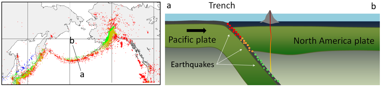
With the development of networks of seismographic stations in the 1950s, it became possible to plot the locations and depths of both major and minor earthquakes with great accuracy. It was found that there is a remarkable correspondence between earthquakes and both the mid-ocean ridges and the deep ocean trenches. In 1954 Gutenberg and Richter showed that the ocean-ridge earthquakes were all relatively shallow and confirmed what had first been shown by Benioff in the 1930s — that earthquakes in the vicinity of ocean trenches were both shallow and deep, but that the deeper ones were situated progressively farther inland from the trenches (Figure 2.13).
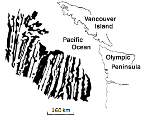
In the 1950s, scientists from the Scripps Oceanographic Institute in California persuaded the U.S. Coast Guard to include magnetometer readings on one of their expeditions to study ocean floor topography. The first comprehensive magnetic data set was compiled in 1958 for an area off the coast of B.C. and Washington State. This survey revealed a bewildering low and high magnetic intensity pattern in sea-floor rocks (Figure 2,14). When the data were first plotted on a map in 1961, nobody understood them — not even the scientists who collected them. Although the patterns made even less sense than the stripes on a zebra, many thousands of kilometres of magnetic surveys were conducted over the next several years.
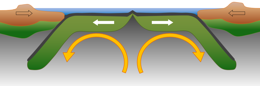
The wealth of new ocean data significantly influenced geological thinking in the 1960s. In 1960, Harold Hess, a widely respected geologist from Princeton University, advanced a theory with many of the elements that we now accept as plate tectonics. However, he maintained some uncertainty about his proposal, and to deflect criticism from mainstream geologists, he labelled it geopoetry. In fact, until 1962, Hess didn’t even put his ideas in writing—except internally to the U.S. Navy (which funded his research)—but presented them mostly in lectures and seminars. Hess proposed that the new seafloor was generated from mantle material at the ocean ridges. That old seafloor was dragged down at the ocean trenches and re-incorporated into the mantle. He suggested that the process was driven by mantle convection currents, rising at the ridges and descending at the trenches (Figure 2.15). He also suggested that the less-dense continental crust did not descend with oceanic crust into trenches, but that colliding land masses were thrust up to form mountains. Hess’s theory formed the basis for the concepts of sea-floor spreading and continental drift, but it did not deal with the concept of the crust being composed of specific plates. Although the Hess model was not roundly criticized, it was not widely accepted (especially in the U.S.), partly because it was not well supported by hard evidence.
The collection of magnetic data from the oceans continued in the early 1960s, but still, nobody could explain the origin of the zebra-like patterns. The first real understanding of the significance of the striped anomalies was the interpretation by Fred Vine, a Cambridge graduate student. Vine was examining magnetic data from the Indian Ocean, and, like others before, he noted the symmetry of the magnetic patterns with respect to the oceanic ridge.
At the same time, other researchers, led by groups in California and New Zealand, were studying the phenomenon of reversals in Earth’s magnetic field. They were trying to determine when such reversals had taken place over the past several million years by analyzing the magnetic characteristics of hundreds of samples from basaltic flows. The Earth’s magnetic field becomes weakened periodically and then virtually non-existent before becoming re-established with the reverse polarity. During periods of reversed polarity, a compass would point south instead of north.
The time scale of magnetic reversals is irregular. For example, the present “normal” event, known as the Bruhnes magnetic chron, has persisted for about 780,000 years. This was preceded by a 190,000-year reversed event, a 50,000-year normal event known as Jaramillo, and then a 700,000-year reversed event.
In a paper published in September 1963, Vine and his PhD supervisor Drummond Matthews proposed that the patterns associated with ridges were related to the magnetic reversals and that oceanic crust created from cooling basalt during a normal event would have polarity aligned with the present magnetic field, and thus would produce a positive anomaly (a black stripe on the sea-floor magnetic map), whereas oceanic crust created during a reversed event would have a polarity opposite to the present field and thus would produce a negative magnetic anomaly (a white stripe). The same idea had been put forward a few months earlier by Lawrence Morley of the Geological Survey of Canada; however, his papers submitted earlier in 1963 to Nature and The Journal of Geophysical Research were rejected. Many people refer to the idea as the Vine-Matthews-Morley (VMM) hypothesis.
Vine, Matthews, and Morley were the first to show this type of correspondence between the stripes’ relative widths and the magnetic reversals’ periods. The VMM hypothesis was confirmed within a few years when magnetic data were compiled from spreading ridges worldwide. It was shown that the same general magnetic patterns were present straddling each ridge. However, the widths of the anomalies varied according to the spreading rates characteristic of the different ridges. It was also shown that the patterns corresponded with the chronology of Earth’s magnetic field reversals. This global consistency provided strong support for the VMM hypothesis and led to the rejection of the other explanations for the magnetic anomalies.
Mid-oceanic spreading
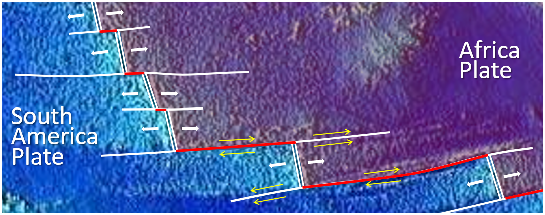
Although oceanic spreading ridges appear to be curved features on Earth’s surface, in fact, the ridges are composed of a series of straight-line segments, offset at intervals by faults perpendicular to the ridge (Figure 2.16). In a paper published in 1965, Tuzo Wilson termed these features transform faults. He described the nature of the motion along them and showed why there are earthquakes only on the section of a transform fault between two adjacent ridge segments. The San Andreas Fault in California is a very long transform fault that links the southern end of the Juan de Fuca spreading ridge to the East Pacific Rise spreading ridges situated in the Gulf of California. The Queen Charlotte Fault, which extends north from the northern end of the Juan de Fuca spreading ridge (near the northern end of Vancouver Island) toward Alaska, is also a transform fault.
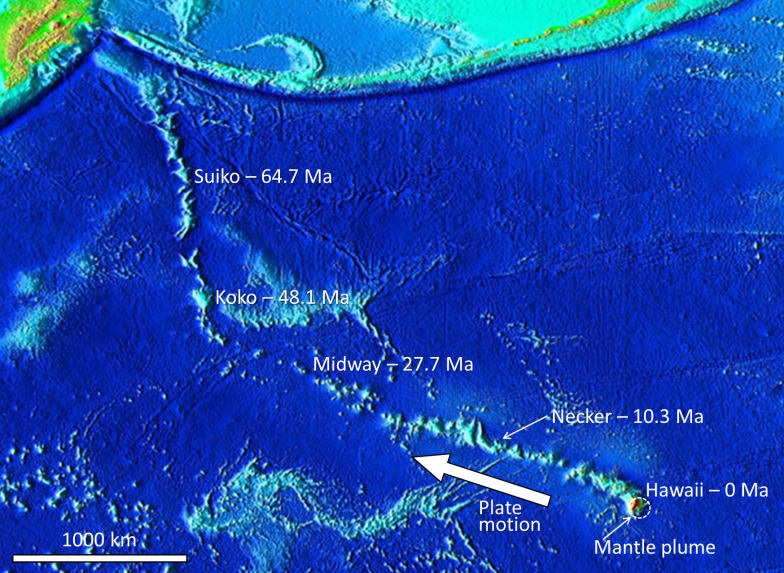
In 1963, J. Tuzo Wilson of the University of Toronto also proposed the idea of a mantle plume or hot spot—a place where hot mantle material rises in a stationary and semi-permanent plume and affects the overlying crust. He based this hypothesis partly on the distribution of the Hawaiian and Emperor Seamount island chains in the Pacific Ocean (Figure 2.17). The volcanic rock making up these islands gets progressively younger toward the southeast, culminating with the island of Hawaii, which consists of rock almost all younger than 1 Ma. Wilson suggested that a stationary plume of hot upwelling mantle material is the source of the Hawaiian volcanism. The ocean crust of the Pacific Plate is moving toward the northwest over this hot spot. Near the Midway Islands, the chain takes a pronounced change in direction, from northwest-southeast for the Hawaiian Islands and to nearly north-south for the Emperor Seamounts. This change is widely ascribed to a change in the direction of the Pacific Plate moving over the stationary mantle plume, but a more plausible explanation is that the Hawaiian mantle plume has not actually been stationary throughout its history and in fact, moved at least 2,000 km south over the period between 81 and 45 Ma. (Source: J. A. Tarduno et al., 2003, The Emperor Seamounts: Southward Motion of the Hawaiian Hotspot Plume in Earth’s Mantle, Science 301 (5636): 1064–1069.)
In the same 1965 paper, Wilson introduced the idea that the crust can be divided into a series of rigid plates, and thus he is responsible for the term plate tectonics.
Volcanoes and the Rate of Plate Motion
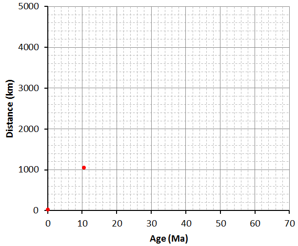
The Hawaiian and Emperor volcanoes shown in Figure 2.17 are listed in the table below, along with their ages and their distances from the centre of the mantle plume under Hawaii (the Big Island).
| Island | Age | Distance | Rate |
|---|---|---|---|
| Hawaii | 0 Ma | 0 km | – |
| Necker | 10.3 Ma | 1,058 km | 10.2 cm/y |
| Midway | 27.7 Ma | 2,432 km | |
| Koko | 48.1 Ma | 3,758 km | |
| Suiko | 64.7 Ma | 4,860 km |
Plot the data on the graph provided here, and use the numbers in the table to estimate the rates of plate motion for the Pacific Plate in cm/year. (The first two are plotted for you.)
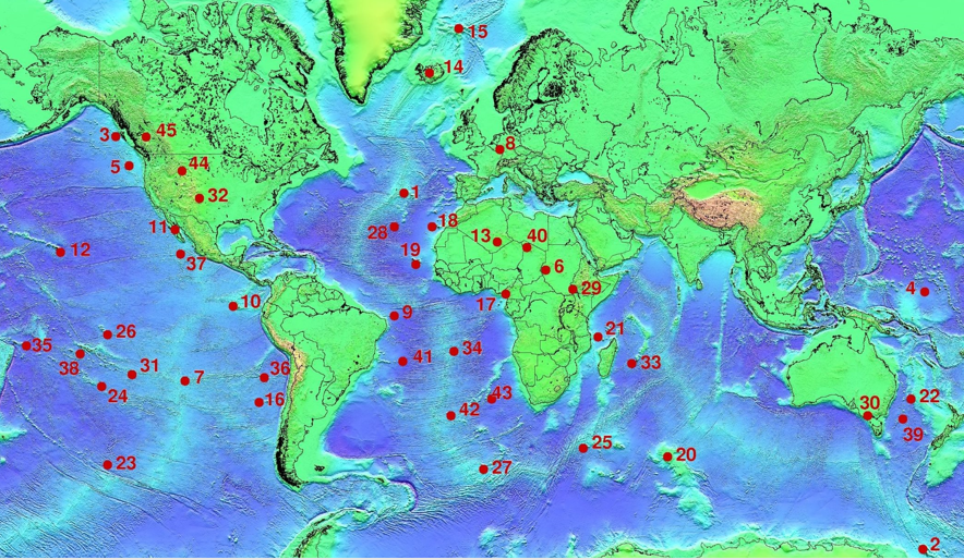
There is evidence of many such mantle plumes around the world (Figure 2.18). Most are within the ocean basins, including Hawaii, Iceland, and the Galapagos Islands, but some are under continents. One example is the Yellowstone hot spot in the west-central United States, and another is the one responsible for the Anahim Volcanic Belt in central British Columbia. It is evident that mantle plumes are very long-lived phenomena, lasting at least tens of millions of years, possibly hundreds of millions of years in some cases.
Paper transform fault model
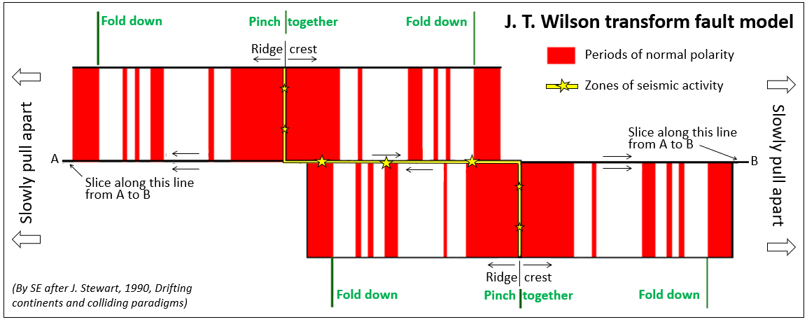
Tuzo Wilson used a paper model, a little bit like the one shown here (Figure 2.19), to explain transform faults to his colleagues. To use this model, either print this page or download the image above and print that, then cut around the outside, and then slice along the line A-B (the fracture zone) with a sharp knife. Fold down the top half where shown, and then pinch together in the middle. Do the same with the bottom half.
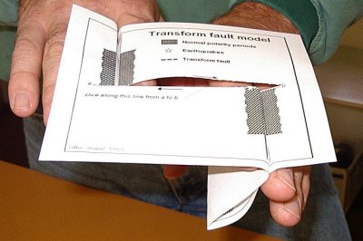
When you’re done, you should have something like the example shown in Figure 2.20, with two folds of paper extending underneath. Find someone else to pinch those folds with two fingers just below each ridge crest, and then gently pull apart where shown. As you do, the oceanic crust will emerge from the middle, and you’ll see that the parts of the fracture zone between the ridge crests will be moving in opposite directions (this is the transform fault) while the parts of the fracture zone outside of the ridge crests will be moving in the same direction. You’ll also see that the oceanic crust is being magnetized as it forms at the ridge. The magnetic patterns shown are accurate and represent the last 2.5 Ma of geological time.
There are other versions of this model available here: Paper Models of Transform Faults. For more information, see Earle, S., 2004, A simple paper model of a transform fault at a spreading ridge, J. Geosc. Educ. V. 52, p. 391-2.
Image Descriptions
Figure 2.8 image description: At 500 Ma, rocks in Europe had upward-pointing magnetic orientations. At 400 Ma, the magnetic orientation levelled. From 300 Ma to the present, rocks in Europe shown an increasingly downward-pointing magnetic orientation. [Return to Figure 2.8]
Figure 2.13 image description: A cross-section of the trench formed at the Aleutian subduction zone as the Pacific plate subducts under the North American plate in the middle of the Pacific Ocean. The farther away an earthquake is from this trench (on the North America plate side), the deeper it is. [Return to Figure 2.13]
Media Attributions
- Figures 2.9, 2.10, 2.12, 2.13, 2.15, 2.16, 2.19, 2.20: © Steven Earle. CC BY.
- Figure 2.11: “Elevation” by NOAA. Adapted by Steven Earle. Public domain.
- Figure 2.14: “Juan de Fuca Ridge” by USGS. Adapted by Steven Earle. Public domain. Based on Raff, A. and Mason, R., 1961, Magnetic survey off the west coast of North America, 40˚ N to 52˚ N latitude, Geol. Soc. America Bulletin, V. 72, p. 267-270.
- Figure 2.17: “Hawaii Hotspot” by National Geophysical Data Center. Adapted by Steven Earle. Public domain.
- Figure 2.18: “Hotspots” by Ingo Wölbern. Public domain.

#/media/File:Hawaii_hotspot.jpg)