3.1 How Do We Define Business Competition?

Perfect Competition, Supply, and Demand

Under a mixed economy, such as we have in Canada, businesses make decisions about which goods to produce or services to offer and how they are priced. Because there are many businesses making goods or providing services, customers can choose among a wide array of products. The competition for sales among businesses is a vital part of our economic system. Economists have identified four types of competition—perfect competition, monopolistic competition, oligopoly, and monopoly. We’ll introduce the first of these—perfect competition—in this section and cover the remaining three in the following section.

Perfect Competition

Perfect competition exists when there are many consumers buying a standardized product from numerous small businesses. Because no seller is big enough or influential enough to affect price, sellers and buyers accept the going price. For example, when a commercial fisher brings his fish to the local market, he has little control over the price he gets and must accept the going market price.

The Basics of Supply and Demand

To appreciate how perfect competition works, we need to understand how buyers and sellers interact in a market to set prices. In a market characterized by perfect competition, price is determined through the mechanisms of supply and demand. Prices are influenced both by the supply of products from sellers and by the demand for products by buyers.

To illustrate this concept, let’s create a supply and demand schedule for one particular good sold at one point in time. Then we’ll define demand and create a demand curve and define supply and create a supply curve. Finally, we’ll see how supply and demand interact to create an equilibrium price—the price at which buyers are willing to purchase the amount that sellers are willing to sell.

Demand and the Demand Curve

Demand is the quantity of a product that buyers are willing to purchase at various prices. The quantity of a product that people are willing to buy depends on its price. You’re typically willing to buy less of a product when prices rise and more of a product when prices fall. Generally speaking, we find products more attractive at lower prices, and we buy more at lower prices because our income goes further.

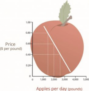
Using this logic, we can construct a demand curve that shows the quantity of a product that will be demanded at different prices. Let’s assume that the diagram “The Demand Curve” represents the daily price and quantity of apples sold by farmers at a local market. Note that as the price of apples goes down, buyers’ demand goes up. Thus, if a pound of apples sells for $0.80, buyers will be willing to purchase only fifteen hundred pounds per day. But if apples cost only $0.60 a pound, buyers will be willing to purchase two thousand pounds. At $0.40 a pound, buyers will be willing to purchase twenty-five hundred pounds.

Supply and the Supply Curve 

Supply is the quantity of a product that sellers are willing to sell at various prices. The quantity of a product that a business is willing to sell depends on its price. Businesses are more willing to sell a product when the price rises and less willing to sell it when prices fall. Again, this fact makes sense: businesses are set up to make profits, and there are larger profits to be made when prices are high.

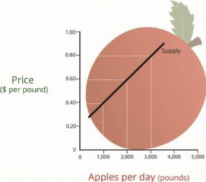
Now we can construct a supply curve that shows the quantity of apples that farmers would be willing to sell at different prices, regardless of demand. As you can see in “The Supply Curve”, the supply curve goes in the opposite direction from the demand curve: as prices rise, the quantity of apples that farmers are willing to sell also goes up. The supply curve shows that farmers are willing to sell only a thousand pounds of apples when the price is $0.40 a pound, two thousand pounds when the price is $0.60, and three thousand pounds when the price is $0.80.

Equilibrium Price

We can now see how the market mechanism works under perfect competition. We do this by plotting both the supply curve and the demand curve on one graph, as we’ve done in the figure below, “The Equilibrium Price”. The point at which the two curves intersect is the equilibrium price.

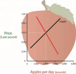
You can see in “The Equilibrium Price” that the supply and demand curves intersect at the price of $0.60 and quantity of two thousand pounds. Thus, $0.60 is the equilibrium price: at this price, the quantity of apples demanded by buyers equals the quantity of apples that farmers are willing to supply. If a single farmer tries to charge more than $0.60 for a pound of apples, he won’t sell very many because other suppliers are making them available for less. As a result, his profits will go down. If, on the other hand, a farmer tries to charge less than the equilibrium price of $0.60 a pound, he will sell more apples but his profit per pound will be less than at the equilibrium price. With profit being the motive, there is no incentive to drop the price.